Hands-on for Toxicity Classification and minimization of unintended bias for Comments using…

Hands-on for Toxicity Classification and minimization of unintended bias for Comments using classical machine learning models

In this blog, I will try to explain a Toxicity polarity problem solution implementation for text i.e. basically a text-based binary classification machine learning problem for which I will try to implement some classical machine learning and deep learning models.

For this activity, I am trying to implement a problem from Kaggle competition: “Jigsaw Unintended Bias in Toxicity Classification”.

In this problem along with toxicity classification, we have to minimize the unintended bias (which I will explain briefly in the initial section).

Business problem and Background:

Background:

This problem was posted by the Conversation AI team (Research Institution) in Kaggle competition.

This problem’s main focus is to identify the toxicity in an online conversation where toxicity is defined as anything rude, disrespectful, or otherwise likely to make someone leave a discussion.

Conversation AI team first built toxicity models, they found that the models incorrectly learned to associate the names of frequently attacked identities with toxicity. Models predicted a high likelihood of toxicity for comments containing those identities (e.g. “gay”).

Unintended Bias

The models are highly trained with some keywords which are frequently appearing in toxic comments such that if any of the keywords are used in a comment’s context which is actually not a toxic comment but because of the model’s bias towards the keywords it will predict it as a toxic comment.

For example: “I am a gay woman”

Problem Statement

Building toxicity models that operate fairly across a diverse range of conversations. Even when those comments were not actually toxic. The main intention of this problem is to detect unintentional bias in model results.

Constraints

There is no such constraint for latency mentioned in this competition.

Evaluation Metrics

To measure the unintended bias evaluation metric is ROC-AUC but with three specific subsets of the test set for each identity. You can get more details about these metrics in Conversation AI’s recent paper.

Trending Bot Articles:

1. Case Study: Building Appointment Booking Chatbot

2. IBM Watson Assistant provides better intent classification than other commercial products according to published study

3. Testing Conversational AI

4. How intelligent and automated conversational systems are driving B2C revenue and growth.

Overall AUC

This is the ROC-AUC for the full evaluation set.

Bias AUCs

Here we will divide the test data based on identity subgroups and then calculate the ROC-AUC for each subgroup individually. When we select one subgroup we parallelly calculate ROC-AUC for the rest of the data which we call background data.

Subgroup AUC

Here we calculate the ROC-AUC for a selected subgroup individually in test data. A low value in this metric means the model does a poor job of distinguishing between toxic and non-toxic comments that mention the identity.

BPSN (Background Positive, Subgroup Negative) AUC

Here first we select two groups from the test set, background toxic data points, and subgroup non-toxic data points. Then we will take a union of all the data and calculate ROC-AUC. A low value in this metric means the model does a poor job of distinguishing between toxic and non-toxic comments that mention the identity.

BNSP (Background Negative, Subgroup Positive) AUC

Here first we select two groups from the test set, background non-toxic data points, and subgroup toxic data points. Then we will take a union of all the data and calculate ROC-AUC. A low value in this metric means the model does a poor job of distinguishing between toxic and non-toxic comments that mention the identity.

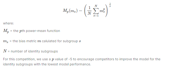
Generalized Mean of Bias AUCs

To combine the per-identity Bias AUCs into one overall measure, we calculate their generalized mean as defined below:

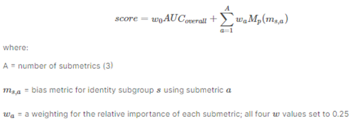
Final Metric

We combine the overall AUC with the generalized mean of the Bias AUCs to calculate the final model score:

Exploratory Data Analysis

Overview of the data

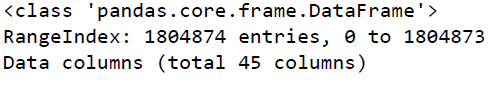
“Jigsaw provided a good amount of training data to identify the toxic comments without any unintentional bias. Training data consists of 1.8 million rows and 45 features in it.”

“comment_text” column contains the text for individual comments.

“target” column indicates the overall toxicity threshold for the comment, trained models should predict this column for test data where target>=0.5 will be considered as a positive class (toxic).

A subset of comments has been labeled with a variety of identity attributes, representing the identities that are mentioned in the comment. Some of the columns corresponding to identity attributes are listed below.

• male
• female
• transgender
• other_gender
• heterosexual
• homosexual_gay_or_lesbian
• Christian
• Jewish
• Muslim
• Hindu
• Buddhist
• atheist
• black
• white
• intellectual_or_learning_disability

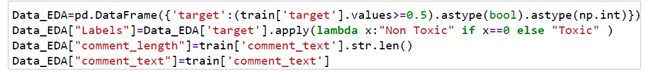
Let’s see the distribution of the target column

First I am using the following snippet of code to convert target column thresholds to binary labels.

Now, let’s plot the distribution

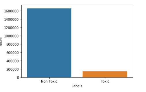
We can observe from the plot around 8% of data is toxic and 92% of data is non-toxic.

Now, let’s check unique and repeated comments in “comment_text” column also check of duplicate rows in the dataset

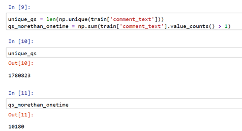
From the above snippet, we got there are 1780823 comments that are unique and 10180 comments are reaping more than once.

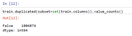
So we can see in the above snippet there are no duplicate rows in the entire dataset.

Let’s Plot box Plot for Non-Toxic and Toxic comments based on their lengths

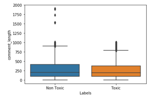
From the above plot, we can observe that most of the points for toxic and non-toxic class comments lengths distributions are overlapping but there are few points in the toxic comments where comment length is more than a thousand words and in the non-toxic comment, we have some point’s are more than 1800 words.

Let’s quickly check the percentile for comment lengths

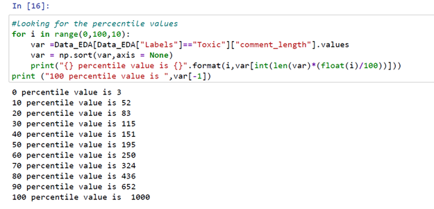
From the above code snippet, we can see the 90th percentile for comment lengths of toxic labels is 652 and the 100th percentile comment length is 1000 words.

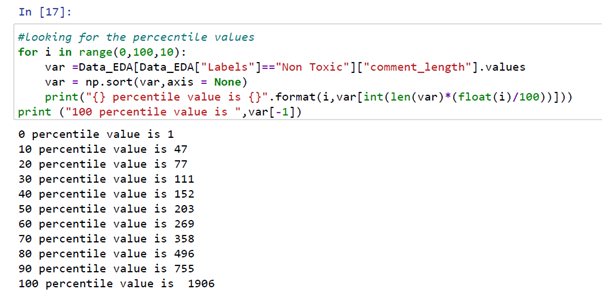
From the above code snippet, we can see the 90th percentile for comment lengths of non-toxic labels is 755 and the 100th percentile comment length is 1956 words.

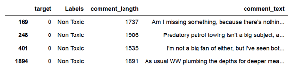
We can easily print some of the comments for which comment has more than 1300 words.

Let’s plot Word cloud for Toxic and Non-Toxic comments

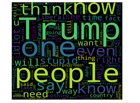
In the above plot, we can see words like trump, stupid, ignorant, people, idiot used in toxic comments with high frequency.

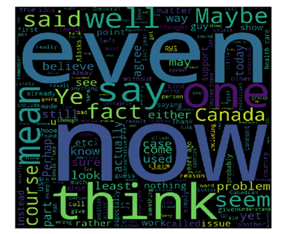
In the above plot, we can see there are no negative words with the high frequency used in non-toxic comments.

Basic Feature Extraction

Let us now construct a few features for our classical models:

• total_length = length of comment
• capitals = number of capitals in comment
• caps_vs_length = (number of capitals in comment)
• num_exclamation_marks = num exclamation marks
• num_question_marks = num question marks
• num_punctuation = Number of num punctuation
• num_symbols = Number of symbols (@, #, $, %, ^, &, *, ~)
• num_words = Total numer of words
• num_unique_words = Number unique words
• words_vs_unique = number of unique words/number of words
• num_smilies = number of smilies
• word_density = taking average of each word density within the comment
• num_stopWords = number of Stopwords in comment
• num_nonStopWords = number of non Stopwords in comment
• num_nonStopWords_density = (num stop words)/(num stop words + num non stop words)
• num_stopWords_density = (num non stop words)/(num stop words + num non stop words)

To check the implementation of these features you can check my EDA notebook.

After the implementation of these features let’s check the correlation of extracted feature with target and some of the other features form the dataset.

So for correlation first I implemented the person correlation of extracted features with some of the features from the dataset and plotted the following the seaborn heatmap plot.

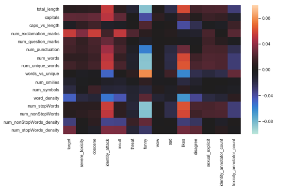
From the above plot, we can observe some good correlations between extracted features and existing features, for example, there is a high positive correlation between target and num_explation_marks, high negative correlation between num_stopWords and funny comments and we can see there are lots of features where there is no correlation between them, for example, num_stopWords with Wow comments and sad comments with num_smilies.

Feature selection

I applied some feature selection methods on extracted features like Filter Method, Wrapper Method, and Embedded Method by following this blog.

Filter Method: In this method, we just filter and select only a subset of relevant features, and filtering is done using the Pearson correlation.

Wrapper Method: In this method, we have to use one machine learning model and will evaluate features based on the performance of the selected features. This is an iterative process but better accurate than the filter method. It could be implemented in two ways.

1. Backward Elimination: First we feed all the features to the model and evaluate its performance then we eliminate worst-performing features one by one till we get some good relevant performance. It uses pvalue as a performance metric.

2. RFE (Recursive Feature Elimination): In this method, we recursively remove features and build the model on the remaining features. It uses an accuracy metric to rank the feature according to their importance.

Embedded Method: It is one of the methods commonly used by regularization methods that penalize a feature-based n given coefficient threshold of the feature.

I followed the implantation from this blog and used the Lasso regularization. If the feature is irrelevant, lasso penalizes its coefficient and make it 0. Hence the features with coefficient = 0 are removed and the rest is taken.

To understand these methods and its implementation more briefly please check this blog.

After implementing all the methods of feature selection I selected the results of the Embedded Method and will include selected features in our training.

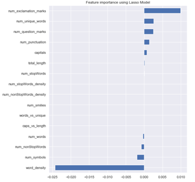
Embedded method mark the following features as unimportant

1. caps_vs_length

2. words_vs_unique

3. num_smilies

4. num_nonStopWords_density

5. num_stopWords_density

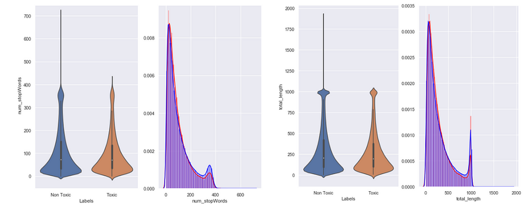
I plotted some of the selected extracted features as the following plots:

Summary of EDA analysis:

1. The number of Toxic comments is less than Non Toxic comments i.e. 8 percent of toxic 92 percent of non-toxic.

2. We printed the percentile values of length of comments and observed the 90th percentile value is 652 for the Toxic and 90th percentile value is 755 for non-Toxic. We also checked there are 7 comments with length more than 1300 and all are non-toxic.

3. We created some text features and plotted the correlation table with Target and Identities Features. We also plotted the correlation table between extracted features Vs extracted features, to check correlation among them.

4. We applied some feature selection methods and used the results of Embedded Method where out of 16 we selected 11 as relevant features.

5. We plotted the Villon and Density plot for some of the extracted features with target labels.

6. We plotted Word cloud for Toxic and Non-Toxic comments and observed some words which are frequently used in Toxic comments.

Now let’s do some basic pre-processing on our data

Checking for NULL values

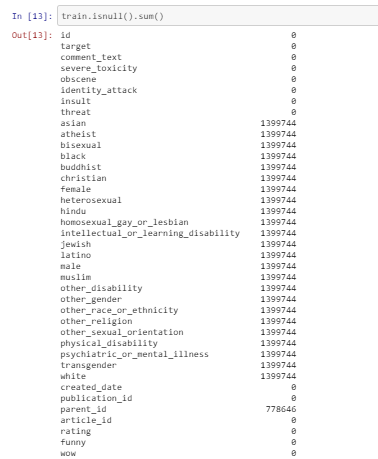
From the above snippet, we can observe there is a lot of identity numerical features with lots of null values and there are no null values in comment text feature. Identity numerical features values are thresholds between 0 to1 along with target columns.

So, I converted the identity features along with the target column as Boolean features as mentioned in competition. Values greater than equal to 0.5 will be marked as True and other than that as False (null values now become False).

In the below snippet I selected few Identity features for our model’s evaluation and converting them to Boolean features along with the target column.

As the target column is binary now our data is ready for binary classification models.

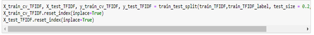
Now I split the data into Train and Test in 80:20 ratio:

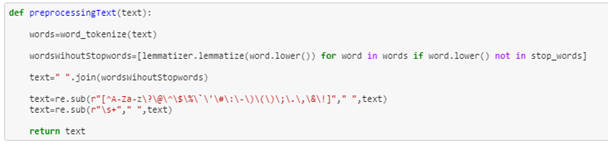
For text pre-processing, I am using the following function in which I am implementing

1. Tokenization

2. Lemmatization

3. Stop words removal

4. Applying Regex to remove all non-words token and keeping all special symbols that are commonly used in comments.

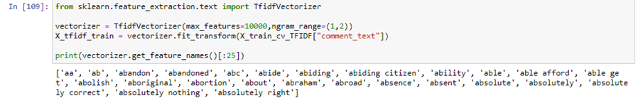
Vectorizing Text with Tf Idf Vectorize

As models can’t understand text directly, we have to vectorize our data. So to vectorize our data I selected TfIdf.

To understand TfIdf and its implementation in python briefly you can check this blog.

So, first, we are applying TfIdf on our train data with maximum features as 10000.

In TfIdf I got the scores for all tokens based on term frequency and inverse document frequency.

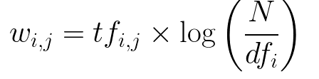
Higher the score more weightage of the token.

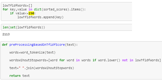
In the following snippet, I collected the tokens along with the TfIdf score in tuples and stored all sorted tuples on the list.

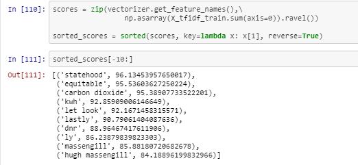
Now based on the scores I selected 150 as threshold and now I will collect all tokens from TfIdf with score greater than 150.

In the following function, I am removing all tokens having a TfIdf score of less than 150.

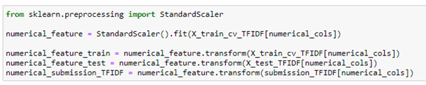
Standardization of numerical features

To normalize the extracted numerical features I am using sklearn’s StandardScaler which will standardize the numerical features.

As I pre-processed the numerical extracted features and text feature lets now stack them using scipy’s hstack as follows:

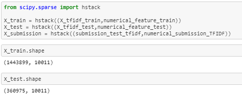
Now our data is ready so let’s start implementing some classical models on it.

Classical models:

In this section I will show you some Classical Machine Learning implementation, to check the implementation of all the classical models you can check my notebook.

Logistic Regression:

Logistic Regression one of the popular classification problems. There is a lot of applications that can be applied using a logistic regression classifier for binary classification problems like spam email filter detection, online transaction fraud or not, etc. Now I will apply logistic regression on the pre-processed stacked data.

To know more about logistic regression you can check this blog.

In the below snippet you can see I am using sklearn’s GridsearchCV to tune the hyperparameters, I choose value 4 for k cross-validation. Cross validations basically used to evaluate trained models with the different values of hyperparameters.

I am using different values of alpha’s get the best score. For alpha value 0.0001 I am getting the best score on CV based on GridSearchCV results.

Next, I trained a logistic regression model with the selected hyperparameter values on trained data, then I used the trained model to predict probabilities on test data.

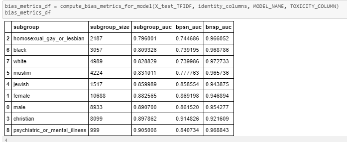
Now I passed the data frame containing Identities columns along with logistic regression probability scores to Evaluation metric function.

You can see the complete implantation of the evaluation metric in this Kaggle notebook.

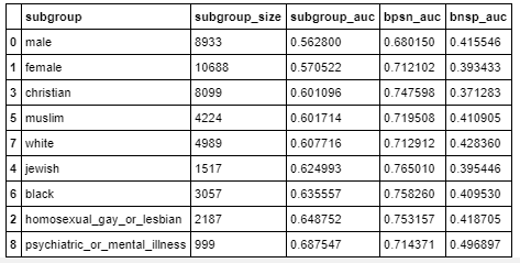
Evaluation metric score on test data: 0.57022

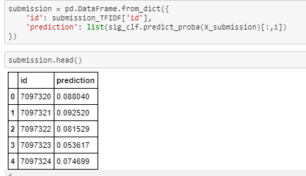
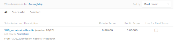
On preprocessing text and numerical features on competition’s train data I preprocessed the submission data as well. Now using the trained model I got probability scores for Submission data as well. Now I prepared submission.csv as mentioned in the competition.

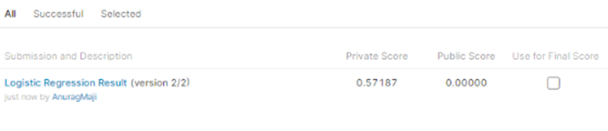
On submitting the submission.csv I got Kaggle score of 0.57187

Now following the same procedure, I trained all classical models. Please check the following table for the scores of all classification models I implemented.

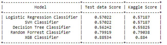
So, the XGB classifier gives the best Evaluation metric and test score among all Classical models.

Please check part 2 of this project’s blog which explains the deep learning implementations and deployment function of this problem. You can check the implementation of EDA and classical machine learning models notebook on my Github repository.

Future work

Can apply deep learning architectures which can improve the model performance.

References

1. https://www.kaggle.com/c/jigsaw-unintended-bias-in-toxicity-classification
2. https://www.kaggle.com/nz0722/simple-eda-text-preprocessing-jigsaw
3. Paper provided by Conversation AI team explaining the problem and metric briefly https://arxiv.org/abs/1903.04561
4. https://www.appliedaicourse.com/
5. https://towardsdatascience.com/feature-selection-with-pandas-e3690ad8504b

Don’t forget to give us your 👏 !

---

Hands-on for Toxicity Classification and minimization of unintended bias for Comments using… was originally published in Chatbots Life on Medium, where people are continuing the conversation by highlighting and responding to this story.